How Oil AI exposes its evidence and limits.
A historically evaluated drilling-screening model for Colorado's DJ Basin — with the passing tests, failed forward tests, and claim boundary shown together. Sections 01–05 walk the Colorado model; section 06 carries the four Texas datasets the same pipeline now runs, the cross-play transfer test, and the coverage guarantees that replaced a hand-tuned uncertainty band.
Open the live evidence view → It shows these
passing and failed checks together with the read-only sealed prediction ledger.
The evidence view, the analyst, and the price feed read the project API; the
public static deploy has no /api routes, so those panels fall back
to the published evidence files instead of failing.
01What "success" means
A well spudded in the modern era (≥ 1999) in an oil/gas/dry-hole class is a success if it produced ≥ 5,000 BOE within 24 months of first production (BOE = oil + gas ⁄ 6); a failure if it produced less or was a dry hole / abandoned location. The rule is frozen and unit-tested, and is censoring-aware — wells too recent to observe a full 24-month window are excluded, not mislabeled.
It's cross-validated by an independent signal: ECMC's own well-class codes. Dry-and-abandoned (DA) and location (LO) wells — the categorical "never a producer" classes — show ~0% production, exactly as the production threshold predicts. Two independent signals agree, so the label isn't an artifact of one choice.
02Why honest validation matters here
This basin is mature and de-risked: the base success rate is 0.86 — operators only drill where they're confident. That makes a naive model look brilliant and hides the real question. Two traps, both closed:
The drilling-density trap
Most of "will this well succeed" is just "are there successful wells nearby." Random train/test splits leak that signal — a well's neighbors land in both sets — and produce fake accuracy. We use spatial-block cross- validation: the basin is gridded into 15 km blocks and entire blocks are held out together. A separate 3 km guard-ring test removes adjacent training wells rather than assuming hashed folds never touch. And we make the density model an explicit baseline (a temporal-safe kNN over neighbor wells) that the real model has to beat.
Temporal leakage
A neighbor contributes only when its complete 24-month outcome was observable before the candidate's exact spud month, and only training-set wells are eligible inside each fold. Same-year future and immature outcomes cannot leak into a prediction.
03Results — model vs. baselines
| Model | AUC | ± | Brier |
|---|---|---|---|
| Majority class | 0.500 | — | 0.133 |
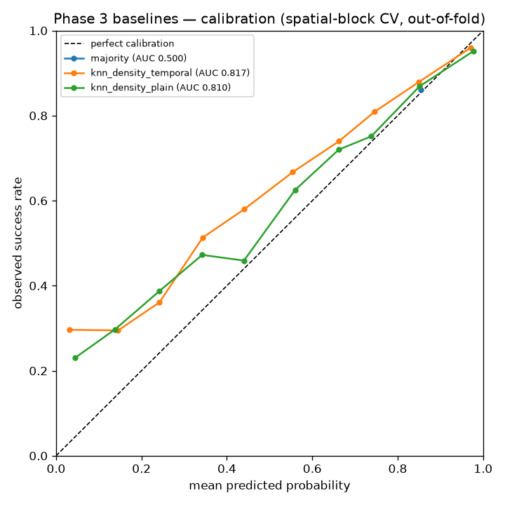
| point-in-time kNN drilling-density | 0.753 | 0.031 | 0.129 |
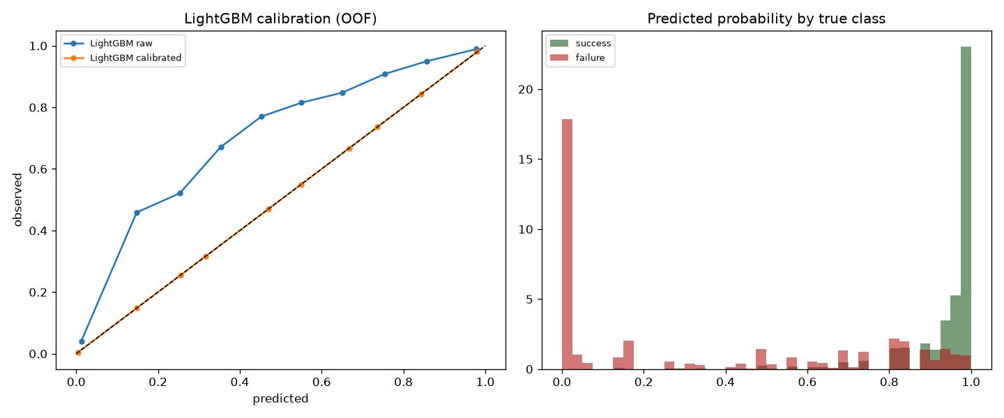
| LightGBM · pre_drill_v1 | 0.842 | 0.021 | 0.081 |
+0.088 AUC over the strict density baseline. This lower, defensible result supersedes the earlier 0.946 score, which included attributes only confirmed after drilling. The production model now uses location, planned vintage/field, and already-observable neighbor outcomes.
Stricter checks: the 3 km-buffered model retains AUC 0.801
versus 0.732 for kNN (+0.069). But fixed 12-month rolling windows average
only 0.622 versus 0.675 for kNN, with positive lift in one of five
windows. Five uniform/recency-weighted candidates failed the promotion gate,
so production remains on pre_drill_v1.
04The basin surface
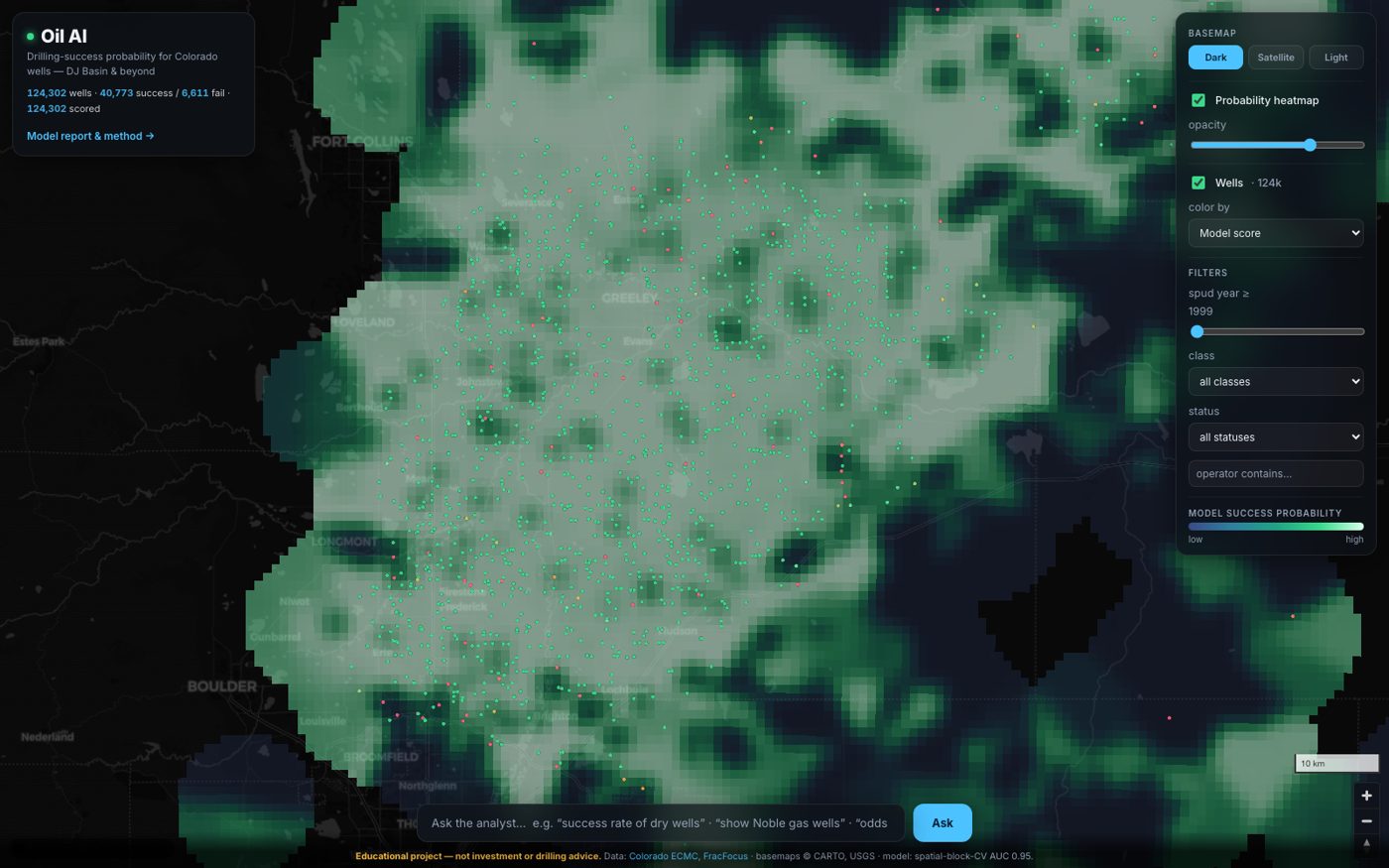
The historically calibrated 5-seed ensemble assigns a screening score to every well and a 1 km grid over the producing footprint — "a well like the local ones, drilled here." The result is a coherent retrospective surface: higher historical scores in the core fading to lower scores at the fringes, with per-cell uncertainty exposed. It is not a validated probability for a future well.
05Limitations (stated plainly)
- Mature, de-risked basin. Base rate 0.86; the hard, valuable prediction is at the fringes and over undrilled locations, not the cored-out center.
- Pre-drill inputs are intentionally sparse. Final depth, producing formation, current class, and completion disclosures are excluded until planned versions of those inputs are available.
- Success-model scope. The classifier has no seismic input and predicts a coarse binary production threshold. Separate DCA, EUR, and economics tools are available, but they are not outputs of this success classifier.
- Density bias. Sparse areas fall back to the base rate — least certain exactly where it'd be most useful. The map now exposes both ensemble uncertainty and an independent high/medium/low geographic-support tier.
- Temporal instability. The spatial score is useful for contemporaneous screening, but next-year ranking is not established and currently trails kNN.
- Displayed score provenance. Validation metrics are spatial out-of-fold, but stored per-well map scores come from the final ensemble refit on all labeled wells. A labeled well's displayed score is therefore in-sample, not its OOF result.
06How it's built & where it runs now
Reproducible from a clean clone: make download-full && make etl &&
make train. Stack: Python · DuckDB · LightGBM · MapLibre · PMTiles ·
FastAPI. Full method in the repo's reports/.
Five datasets, four basins — one model each
Colorado is no longer the only pipeline. The same frozen label rule, the same spatial-block cross-validation, and the same point-in-time density baseline now run over Texas Railroad Commission data in four more datasets, covering 167,678 scored wells in all. Each one gets its own model and its own baseline — nothing is pooled to flatter an average, and no two plays ever share a success threshold. Every figure below is a historical screening result; none of them is a validated future-well probability.
| Dataset | Wells | Model AUC | Density baseline | Forward / temporal test |
|---|---|---|---|---|
| CO · DJ Basin (oil & gas) | 124,302 indexed | 0.842 | 0.753 | 0.622 vs 0.675 — promotion blocked |
| TX · Eagle Ford gas | 5,538 scored / 4,958 trainable | 0.8804 | 0.7544 | 0.841 vs 0.789 |
| TX · Delaware gas | 9,411 scored / 7,209 trainable | 0.9033 | 0.7328 | 0.800 vs 0.637 |
| TX · single-lease oil | 6,085 scored / 4,516 trainable | 0.9056 | 0.764 | 0.836 vs 0.739 † |
| TX · Barnett gas ‡ | 22,342 scored / 18,960 trainable | 0.8864 | 0.7503 | 0.9601 vs 0.8064 ‡ |
† The oil back-test window has a base rate of 0.877 — most wells in it succeeded. AUC is prevalence-invariant, so that does not inflate the number, but the thin negative class makes it a noisy estimate and any accuracy-style reading of it would be flattered. The caveat travels with the figure wherever it is quoted.
‡ The Barnett is modelled, scored and gated but is not yet exposed in the map, terminal or 3D views. Its forward figure is the highest here and the least load-bearing: Barnett drilling collapsed after the gas-price era that built the play, so a 2020 cutoff leaves only 224 test wells — 1.2% of the trainable cohort, at a 0.772 base rate. Read it as encouraging and under-powered. It is also the play where FracFocus reaches only ~12% of trainable wells, so geography, operator identity and lateral length carry it.
Texas · Eagle Ford gas
Gas first, because Texas reports oil by lease while a single-well gas lease gives a clean per-well series. 5,538 wells are scored and 4,958 labeled under the maturity and left-censoring guards, and the model is calibrated to AUC 0.8804 against a 0.7544 point-in-time density baseline (+0.126). The lift was built one feature family at a time: location + vintage (0.8308), county and district (0.8327), pre-production operator and field/reservoir attributes (0.8481), FracFocus frac size and depth plus neighbour features (0.8709), and finally lateral length (0.8819). Leave one family out and lateral is the one the model misses most — +0.0110 AUC, ahead of operator/field at +0.0105 — see below for why it turned out to be free. Proppant-per-foot stays out: recoverable from FracFocus, but only 37% covered and collinear with the frac-water feature already present. A cutoff-2020 forward split holds at 0.841 versus 0.789 for density, but the county detail is where the honesty lives: only La Salle shows a statistically resolved forward edge; Karnes and De Witt are consistent with zero lift over density at these sample sizes.
Texas · Delaware gas
The same recipe transfers west. 9,411 Delaware Basin gas wells are scored and 7,209 are trainable after the maturity and censoring guards. The model reaches AUC 0.9033 against a 0.7328 density baseline — +0.1705, the largest historical lift in the project — and unlike Colorado it survives a forward split, at 0.800 versus 0.637 for density. Frac water volume, true vertical depth, and position lead the feature ranking, the same ordering the Eagle Ford model found.
Texas · single-lease oil, and the allocation wall
Oil in Texas is a measurement problem before it is a modelling problem. The RRC reports oil production per lease, and the completion snapshot carries no spud or completion dates, so any per-well oil series on a multi-well lease is an allocation rather than a measurement. We measured that error instead of assuming it away: a static equal split carries a median per-well error of 50% on two-well leases, rising to 91% on five-well leases, and even an oracle that knows exactly when each well produced still leaves 24–36% — the residual is rate heterogeneity between wells producing side by side, which no timing source fixes. So multi-well-lease oil is excluded by design. Only true single-well leases, where the lease series is the well series, are labeled: 6,085 scored, 4,516 trainable, AUC 0.9056 against a 0.764 density baseline (+0.1416). The cutoff-2020 forward split gives 0.836 versus 0.739 for density — with the 0.877 base-rate caveat above — and the per-play forward picture is uneven: Delaware 0.735 vs 0.693, Eagle Ford 0.818 vs 0.721.
Does it learn geology, or memorise a play?
The sharpest criticism of any spatial well model is that it may be a density map in a trenchcoat — a lookup table that memorised which corner of the basin is good. Every figure above is measured with train and test wells drawn from the same play, so none of them can settle it. So we tested it directly: train on one Texas play, score a different play's held-out wells, with no target-play labels reaching the model at all — seven numeric features (vintage, depth, frac water, frac-job count, lateral, log-lateral, water-per-foot), no coordinates, no neighbour success rates.
Mean transfer AUC 0.8181 against a mean in-play ceiling of 0.864 — 87.2% of skill retained across a basin boundary — and 11 of 12 directed pairs beat the target play's own density baseline. The decomposition is the interesting part: crossing phase at fixed basin retains 0.926 of in-play skill, crossing basin at fixed phase only 0.816. Gas and oil wells in the same rock are drilled and completed alike; rock is what does not travel.
Two things this does not mean. Every transfer sits below its in-play ceiling (mean −0.046 AUC), so a play's own wells remain worth more than a foreign play's. And one direction fails outright: a Delaware-trained model scores Eagle Ford gas at 0.6989 — worse than that play's density baseline, because the Eagle Ford is the oldest and deepest cohort and the Delaware's splits are calibrated on shallower, newer, longer wells. Rank-normalising each feature to its within-play percentile repairs that case at no cost to the average. Four cohorts in two Texas basins is a narrow universe; the claim is "transfers within Texas unconventional plays", not "transfers anywhere".
The feature we said was paywalled, and wasn't
Earlier versions of this page said lateral length and proppant-per-foot "stay out because they are paid data". Half of that was wrong. The Texas Railroad Commission publishes directional-line geometry openly, so a per-well lateral can be reconstructed for 167,056 wells across 221 counties — 34,824 of them inside the modelled plays — at a 100% exact-coordinate join, with the units proved to be feet by regressing geodesic path length against the published value (slope 1.002, R² 0.999996) rather than assumed. It is now the single most valuable feature family in the platform.
The caveat is part of the finding: what the geometry yields is surface-to-bottom-hole displacement, biased upward by the build section (order +500–1,000 ft). An excellent relative driver; a biased absolute number; never published as a completed-lateral statistic.
The same geometry settled something nobody here had asked: every Texas well coordinate in this project is a bottom-hole location, sitting within a median 7 ft of the far end of the lateral and a median 7,670 ft (1.45 miles) from the pad — a gap that has widened every vintage. It is not a shift you could subtract out, because laterals run in both directions off a pad: the mean offset nearly cancels while the median per-well offset is 2,511 m. Rebuild a 10-nearest-neighbour graph on surface coordinates instead and half of every well's neighbour set changes. No model changed — the inputs are identical — but the meaning is now documented and gated. Map dots are correct for reading geology and mislabelled as infrastructure: a well's dot can sit 1.5 miles from its rig.
What "uncertain" now means
Each scored well ships a score_std — the spread of a five-seed
ensemble. It was a dispersion number with no coverage meaning: there was
no level at which "score ± std" was claimed to contain anything, and none had
been measured. The EUR band was worse — its upper quantile had been hand-tuned
off nominal precisely because the nominal fit under-covered.
Both are now replaced by conformal prediction, which gives distribution-free coverage by construction — but only under exchangeability, which spatially dependent wells violate. So every experiment runs twice: once with calibration and test in different 15 km spatial blocks (the honest setting, quoted here) and once on random splits (the control). The gap between them is the price of spatial dependence, measured rather than assumed. At a 90% target, Eagle Ford gas covers 0.8911 of held-out wells under spatial blocks and commits to a single label on 79% of them.
The sharpest result is a warning. A marginal 80% guarantee is kept by
over-covering the wells the ensemble agrees on and under-covering the ones it
does not — to 0.5542, barely half the promised rate, in the highest
score_std third. Calibrating separately within each third restores
it. So the heuristic was never wrong; it was unused. Anyone applying a
coverage claim to one slice of a play should expect the worst-slice number, not
the headline.
What is still not established
All five results are back-tests over already-drilled wells, chosen by operators who knew things this model does not. Forward tracking is wired and has now placed its first real bet: 762 pending Colorado permits are scored under the pre-drill contract and frozen by a manifest pinning the scoring date and the checksums of both the model and the scored file, alongside the dated Colorado permit feed (763–779 permits depending on the snapshot, plus archived snapshots), 2,373 Texas permit positions, and a keyless FRED price feed.
Read that board as a queue, not a forecast. Colorado's forward test is documented weak — rolling-origin evaluation gives AUC 0.622 against a 0.675 density baseline, positive in only 20% of windows — and being point-in-time honest about the features does not repair that. Two constraints are built into the board itself: 41 low-support permits carry no rank at all rather than a manufactured number, and the board states plainly that its top is not distinguishable from its middle, because 91% of supported permits score above the base rate. The information is at the bottom of the board.
Elsewhere on the site, the completion-design response curves answer "what does another 2,000 ft buy me here?" using the exact ensembles the map is scored from — and they are not causal. Comparing only wells drilled in the same year as each other erases 23–57% of the apparent value of length, because long wells are new wells. Read those curves as an upper bound on what length is worth, never as a forecast.
Educational project — not investment or drilling advice. Colorado and Texas data are provided by those states "as is", without warranty; used here at the author's own risk.